Home
/ How To Remove Pivot Table Format : Select the menu and choose the entire pivot table.
How To Remove Pivot Table Format : Select the menu and choose the entire pivot table.
How To Remove Pivot Table Format : Select the menu and choose the entire pivot table.. Below are the steps to delete the pivot table as well as any summary data: In the ribbon, select table design > table styles and then click on the little down arrow at the bottom right hand corner of the group. Click in the pivot table. Tip #10 formatting empty cells in the pivot. In case your pivot table has any blank cells (for values).
Clearing a check box in the field list removes all instances of the field from the report. You may need to scroll to the bottom of the list. Click edit rule, to open the edit formatting rule window. Also check autofit column widths on update, if you need. Go to conditional formatting and click on create a new rule.
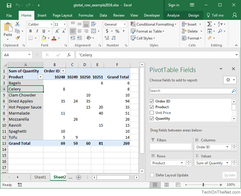
Ms Excel 2016 How To Remove Row Grand Totals In A Pivot Table from www.techonthenet.com Go to conditional formatting and click on create a new rule. Then, i refreshed the pivot table, and the only formatting that disappeared was the fill colour in cell d5, where the f4 shortcut had been used. After you paste the pivottable as values, go to the original pivottable, highlight it, press format painter button, and then paint the second pivottable! Go to conditional formatting tab. To prevent it happening in future go to file > options > data and tick disable automatic grouping of dates. Date formatting in a pivot table. If you get a cannot change this part of a pivottable report message, make sure the entire pivottable is selected. You can use the format painter to grab the format to the second instance of the pivottable.
Intermediate download the excel file.
Here we have a table of product orders and sales from january to february, with corresponding %sales. Now copy the entire pivot table data by ctrl+c. Intermediate download the excel file. Give this a try and see if it works. Select the menu and choose the entire pivot table. Undertaking below steps is supposed to solve this issue (but as i said even this control is not 100% successful) right click on a pivot. To turn this setting off: Applying conditional formatting to remove blanks. Click to uncheck the (blank) check box. Press ctrl+a, and press delete again. Date formatting in a pivot table. Pivot table background cell color. To prevent it happening in future go to file > options > data and tick disable automatic grouping of dates.
Select any cell in your pivot table, and right click. Click in the pivot table. If you're using a device that doesn't have a keyboard, try removing the pivottable like this: Click on the pivot table so that you can see the pivot table contextual tabs. Learn how to apply conditional formatting to pivot tables so that the formats are dynamically reapplied as the pivot table is changed, filtered, or updated.
How To Delete A Pivot Table In Excel Easy Step By Step Guide from v1.nitrocdn.com Hi all, i have a pivot table in excel 2007. Then, i refreshed the pivot table, and the only formatting that disappeared was the fill colour in cell d5, where the f4 shortcut had been used. The pivot table is unlinked, but if you use excel 2007 or excel 2010, the fancy pivot table style formatting is gone: To apply conditional formatting to remove blanks in a pivot table: Then choose pivottable options from the context menu, see screenshot: To turn this setting off: On the layout & format tab, in the format options, remove the check mark from autofit column widths on update. In the list of rules, select the data bar rule, which applies to cells b3:b8.
Undertaking below steps is supposed to solve this issue (but as i said even this control is not 100% successful) right click on a pivot.
Select classic pivottable layout (enables dragging of fields in the. Press ctrl+a, and press delete again. When i do this though, excel strips out all of the pivot tables formatting like bolded column headings and colors, and lines delineating the sections of the table. Next highlight either the entire visible window or specific cells that the pivottables fall on. Also check autofit column widths on update, if you need. When you double click on a value in a pivot table to see the detail behind it, excel automatically shows the data in a table format. Select any cell in the pivot table click on the 'analyze' tab in the ribbon. Intermediate download the excel file. Then choose pivottable options from the context menu, see screenshot: Below are the steps to remove the excel table formatting: Give this a try and see if it works. Select the range of cells that we want to analyze through a. Click to uncheck the (blank) check box.
Next highlight either the entire visible window or specific cells that the pivottables fall on. To get the formatting back, you need to perform two additional steps: In the list of rules, select the data bar rule, which applies to cells b3:b8. Go to conditional formatting tab. Select specific text from the dropdown list of format only cells with.
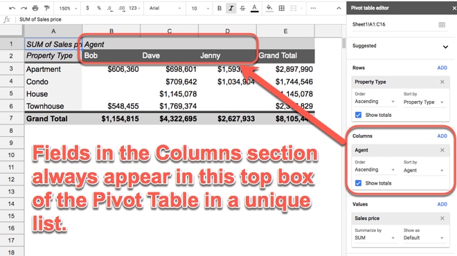
Pivot Tables In Google Sheets A Beginner S Guide from www.benlcollins.com Select the new rule option. Select any cell in the excel table click the design tab (this is a contextual tab and only appears when you click any cell in the table) in table styles, click on the more icon (the one at the bottom of the small scrollbar Go to conditional formatting and click on create a new rule. Sometimes the list doesn't look the way you'd like it to, and the numbers aren't formatted the way they are in the source data. At the top of excel, click the file tab. If you're using a device that doesn't have a keyboard, try removing the pivottable like this: In the pivottable field list, clear the check box next to the field name. Pivot table background cell color.
Right click on the pivot and go to pivot table options;
In the data options section, add a check mark to disable automatic grouping of date/time columns in pivottables. Format cells dialog box will open. Go to conditional formatting tab. Surprisingly, the fill colour was still in e5, even though it was a copy of the d5 formatting. On the ribbon's home tab, click conditional formatting, then click manage rules. This is a contextual tab that appears only when you have selected any cell in the pivot table. Undertaking below steps is supposed to solve this issue (but as i said even this control is not 100% successful) right click on a pivot. Sometimes the list doesn't look the way you'd like it to, and the numbers aren't formatted the way they are in the source data. Below are the steps to delete the pivot table as well as any summary data: In the list of rules, select the data bar rule, which applies to cells b3:b8. In the pivottable options dialog box, click layout & format tab, and then check preserve cell formatting on update item under the format section, see screenshot: Right click on the pivot and go to pivot table options; To select the table, go to analyze tab;
When you double click on a value in a pivot table to see the detail behind it, excel automatically shows the data in a table format how to remove pivot table. Learn how to apply conditional formatting to pivot tables so that the formats are dynamically reapplied as the pivot table is changed, filtered, or updated.